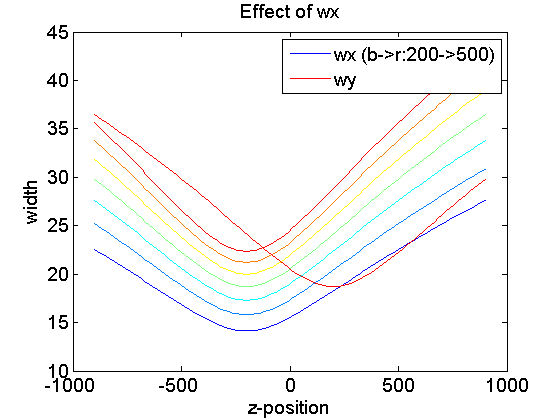
Curves fit the following polynomial:
where
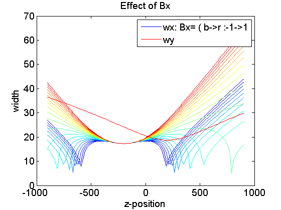
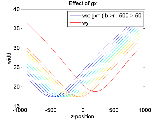
In general we will require $latex gx$ to be negative $latex gy$ to be positive. $latex Ax$ and $latex Bx$ are correction factors and should be small. See Exploring Zcal Pars below for more information. It might be good to consider bounding these to reasonable ranges during the fitting.
As described in the previous post, to compute the calibration curve from data, we simply need to know where are beads are in z, and what there width are. The second criteria we measure directly during the calibration movie (or any movie). The first point is not as simple as it seems, because even though we take a calibration movie at known stage positions, the slide will always have some finite tilt, and thus not all the beads are in that same plane. There is a minor issue too that stage 0 will never correspond exactly to focal plane = 0. But for a single channel we don’t need to worry about where we zero the z-axis anyway. We will return to this when we do multicolor calibration next.
So we begin by taking a calibration movie (recorded using the calibration mode in the piezo stage / focus-lock controller on our system), which just shoots ~300 frames of beads stepping uniformly from -600 nm to 600 nm, with the first and last ~20 frames recorded at position ‘0’. (Note: some setups record in the opposite direction, this does not matter). Also because of z-drift the actual position may go from -600 to 500 or 700. This does matter, but as long as we know the true bead position it should not be a problem that our scan space is non-uniform. It seems most people use the programmed step size position rather than the recorded one, but I think we can get this back out.
Then we fit these beads using our best guess parameters for the z-calibration curve. We also get the true width for each bead (or average width and axial ratio, from which we can compute $latex wx$ and $latex wy$ as $latex wx = w/ax$ and $latex wy = w*ax$). We use the estimated z-positions to compute a sample plane for the beads, from which we correct each beads stage position throughout the recording.
Now 2 things can happen. Our calibration either underestimates the degree of tilt, because the best guess curve was too shallow, or overestimates it. If we underestimate it, things look like this: 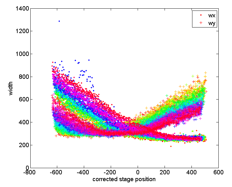
For now, ignore the color. Observe that all the dots (or pluses for $latex wy$) don’t line up along a common curve. This is because they are not in fact running over the same range of z-values — some of these beads went through a range shifted further below focus and some through a range shifted further above focus. This becomes evident if we actually trace individual beads (all localizations from a given bead are plotted in the same color).
If the calibration / tilt correction over-estimates the tilt things look like this: 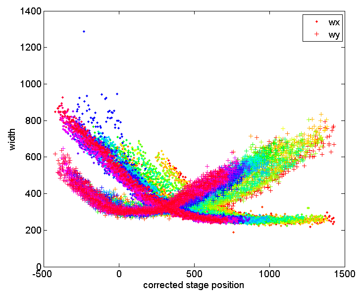
If we ignore the color, once again, it looks like we just have a poor fit scatter. But what actually happened is evident in the colored profiles: some individual curves that should line up are just shifted too far left and right because we have overestimates how different are the z-ranges that they went through.
The existing approach fits a curve to the whole mess (indepedent of bead identity), and then uses a window to choose ‘good beads’ to estimate a new curve. Ideally these are the ones that are displaced the least from true zero (if the window is tight), and when the new fit curve is iterated to refit all the beads the tilt will be estimated better and the points will start to converge more along the line.
This does converge somewhat and give reasonable fits in practice. However I don’t believe that it actually converges to the accuracy of the data. The best fit curves through the two clusters shown above don’t obviously converge to the correct one. Like, how does this algorithm actually behave if it’s far away from the correct fit. How does it behave when its close? Does it get monotonically closer (doesn’t seem to in my experiments). Over many iterations, is it converging faster at the beginning or the end? Also refitting all these beads is probably the slowest step in the algorithm so maybe we don’t want to do that hundreds of times (especially if your algorithm is to repeat each by hand…).
By better using the available data from linked beads, it appears that the ‘correct’ curve is simply the translation that aligns the individual curves for all the beads. e.g. something like this: 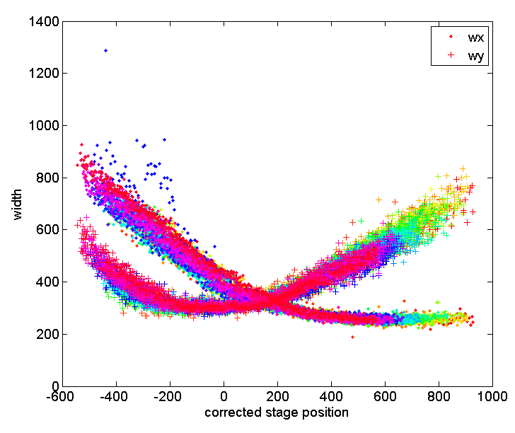
So the algorithm should just compute this optimal curve shift. I’m sure there’s a good fast way to do this with SVD or something, and that I’ve done it before. I just need to figure out how to implement this step.
Then compute the curve fit on the REGISTERED curves from INDIVIDUAL BEAD TRACES. At the next iteration this should give the correct tilt and everything should match easily.
Exploring Zcal Pars: