10:00 A – 7:40P, 8:30P-10:30P
Genomics
- processing real vanSteensel data now
- Reading in data and converting to int8 data matrix for data compression.
cellfun(@(x) int8(round(20*str2double(x))), data) - seems to be running slower than looping the over the columns…
- Actually need single to be able to call PCA, and need to covert output components to double to enable plotting the data axis on the PCs.
- Anyway, this works, calls the HMM as expected, data look good:
- States follow Pc as expected.
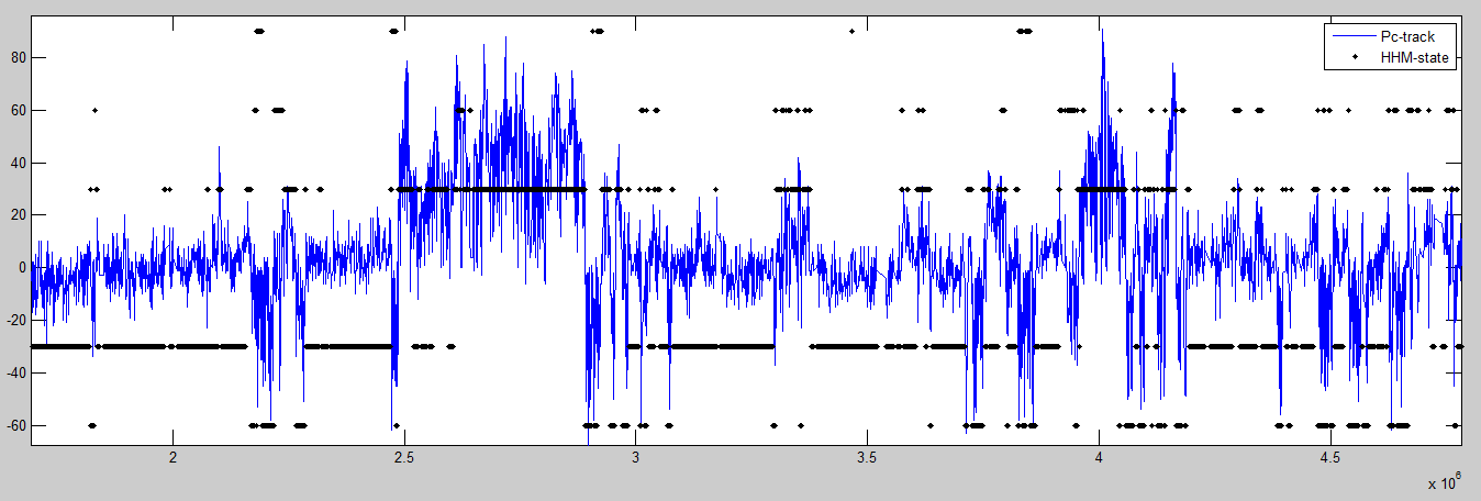
-
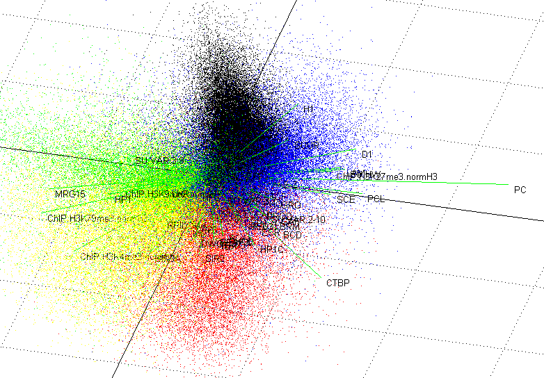
I think I correctly guess all the state types from this Pc plot to put the colors right:

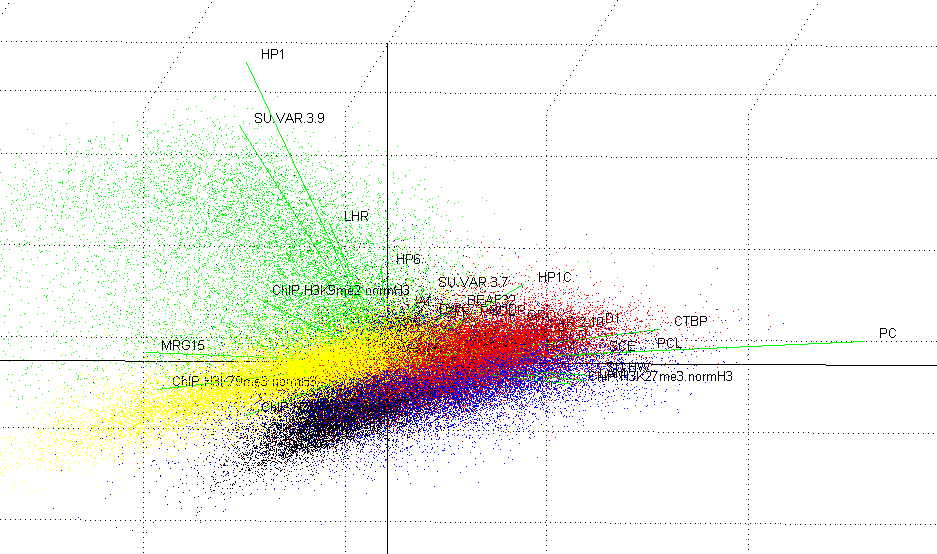
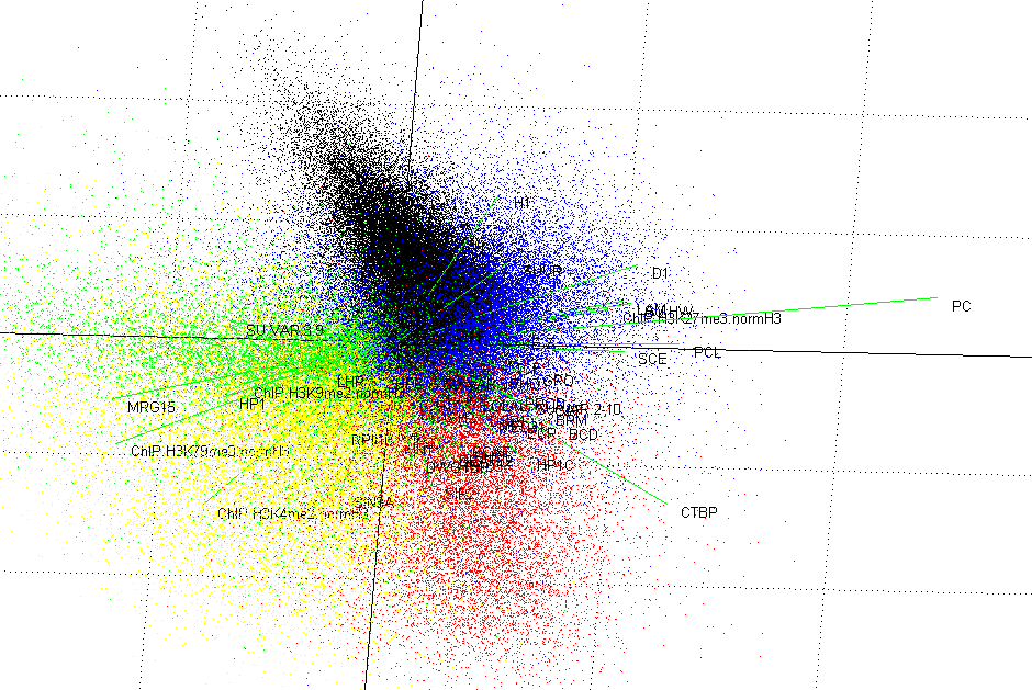
Original paper:
to Re-do probe design: pasting homology-free 20mers together to make 64mers is not a good approach for building homology free 64mers. 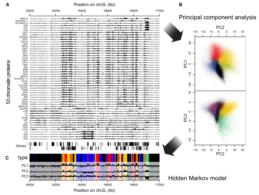
Now Adding noise and seeing the effect
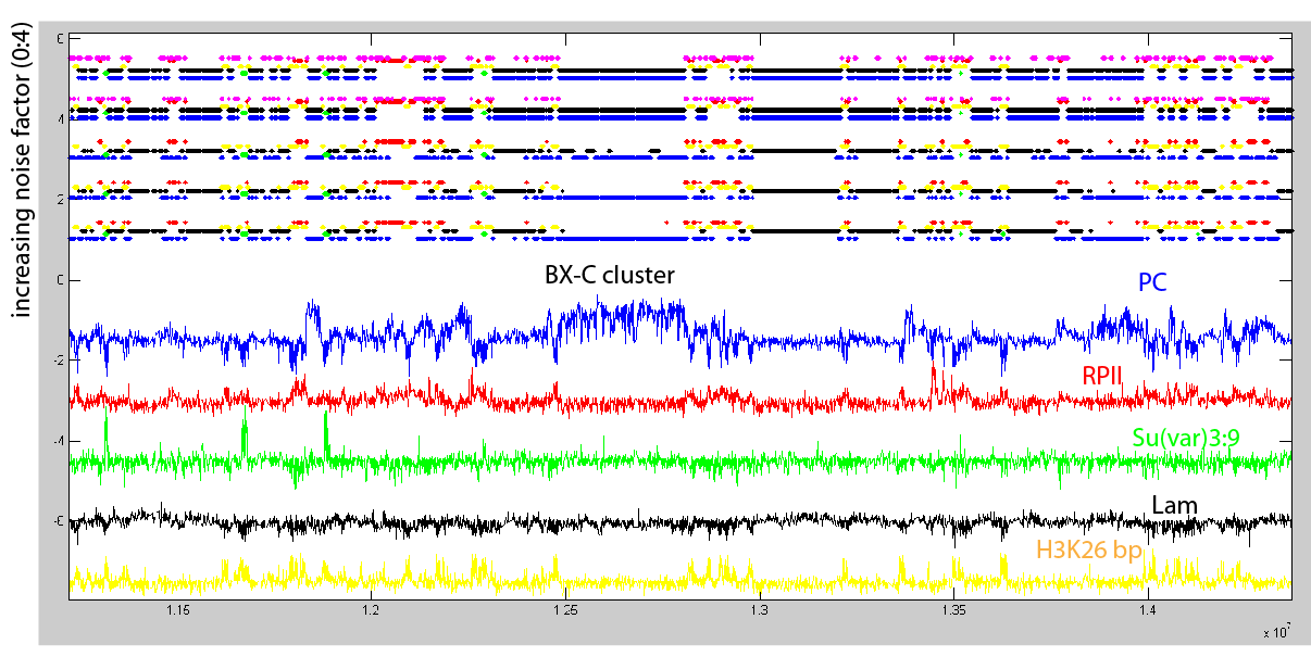
The top tracks show the state classifications as determined by the HHM model with 5 states. The colors are assigned to the state based on the presence of the dominant marks associated with that state. Below these state classfications I’ve plotted the DAMID chip tracks for a single ‘dominant mark’ of each class, color coded appropriately.
The lowest state classification (just above the chip-tracks) is the HMM model on the “raw” data. This should be the same classification as produced by the original model. The successive tracks above have noise added to the raw DAMID chip tracks prior to running the HMM classifier. Most chip tracks range from -4 to 4, the noise added is uniform between -n and n, where n goes from 0 to 4 in the successive tracks.
Observations:
- The most salient change is that as noise increases the HMM starts assigning anything that was previously black or blue to be a common state, and adds a new state. This looks like a new state of active chromatin. Might be worth running the original classifier with 6 or 10 states and see how the clusters look.
- Actually, close inspection of the new state to the left shows that what was previously Pc DNA has been split into the new state or the black state: The first mega-base before the BX-C cluster has most of what was called ‘BLUE’ chromatin in the no-noise case classified as the new state. HOWEVER, the ‘true’ Pc-target regions (SS, BX-C) are all classified as BLACK.
- These seem to be mostly Pc-regions interspersed with red-yellow chromatin = magenta
- Certainly we should at least consider them low-confidence blue regions (our initial goal), since they switch state relative to high confidence regions.
- somewhat surprisingly (I think) the yellow red classification is rather robust.
- Some Green regions do get lost (those to the right of the BXC), which fits with expectations looking at the Su(var)3:9 track that these are not strong green regions.
Other thoughts
Polycomb does have some preference for simply repressing off chromatin — hence the massive largely inactive regions of the genome that are not ‘GREEN’ classic constitutive heterochromatin, show clear enrichment for polycomb signals. Still, this ‘signal is dramatically less than for confirmed polycomb target genes (ones whose expression clearly changes in direct response to PcG mutations).
** Smaller noise step, more rounds of fitting ** 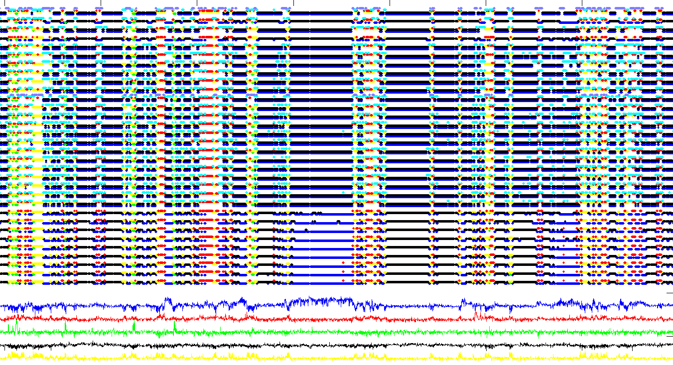
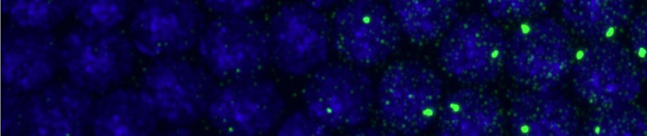
STORM Analysis
- Dotfitting still running on Tuck and Cajal, but almost finished.
- Analysis finished.
- Launched dot-clustering scripts on new BX-C S2 cell data for S2 vs. S3 cell comparison (previous S2 dataset was a bit small).
- Launched dot-clustering script on all new Fab7 data. Will probably need some better data filtering for a sharper dataset, but we’ll see where the rough automatic version stands.
- To improve in clustering
- get rid of non-switching clusters near image edge
- get rid of ultrabright clumps of dye on small dead cells.
- Should add a get Mosaic call to these scripts
- Need to call the correct conventional image in order to use conventional mask! Using out of plane image (first or last) creates serious problems (obviously)!