9:45 A – 7:25 P, 8:30 – 11:00 P
Modeling
- Peccoud’s solutions for the two state model do have the correct form as backward reactions go to zero.
- check these solutions with Sanchez’s approach.
- Also still correct
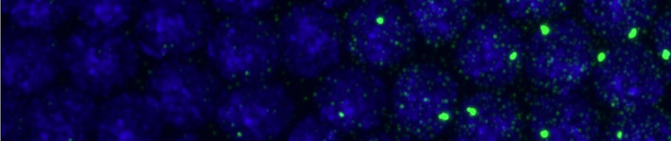
En embryo data
- overlaying mosaics: best to do first at low resolution
- need to make sure entire mosaic is converted
- quickstart needs to be deleted to re-initialize when new converted .mat files are added to mosaic.
fid = fopen(‘H:\2013-07-25_EnEmbs\C2_Mosaic2\mosaicNew.msc’,’wt+’); % the t here means open in text format and is CRITICAL for python to make sense of these text/msc files.
for i=1738:2484
fprintf(fid,[‘mosaic_’,num2str(i),’.stv’]);
fprintf(fid,’%s\r\n’,”);
end
fclose(fid);
Schier Lab collaboration
- group meeting, 3:45 P – 7:15 P
Modeling
- Possible fix for variance?
I also slipped in my algebra before: taking the limit of the solutions I get from your approach as the reverse reaction rates go to zero, still gives the correct answer in the case of simple models where I can compute the moments by other means. For example:
Let the rate matrix K =
[k1, -k1, 0
k2, -k2-k3, k3
0, k4, -k4]
(using the standard convention in probability that the rows of the rate matrix sum to zero),
and let r = [0,0,kt]
Evaluating this system as k2 -> 0, we recover the moment distributions of the two state promoter, which is exactly what should happen if the system can leave but never return to state 1. It also appears to me there is nothing intrinsically wrong with the using this approach on the cyclical state.
For example, if the states are connected like:
  (1) --> (2) --> (N)
   ^               |
   |_______________|
K =
[-kf, kf, 0, 0
0, -kf, kf, 0
0, 0, -kf, 0
kf , 0, 0, -kf]
and as long as the system sits state (N), it produces mRNA at rate kt (which decays at rate d).
Certainly we get the expected mean correct (this thing spends 1/N of its time in state N producing mRNA at rate kt, and so the mean mRNA levels are just kt/(N*d))
Having made this check, it seems one should be able to set up the a system to check the effect of length still using your approach. Part of the trick, as you allude to in your previous message, is just being sure to balance the other variables appropriately, since multiple aspects of the system change as the number of transition states in the return pathway are changed. I agree simply adding states should increase CV, since the system spends more time in OFF states and the mean decreases (decreased activation frequency). In fact both the mean and the standard deviation decrease with N, but the mean decreases as 1/N and the stdev as 1/sqrt(N). This is analogous to the transition times, where the mean time increases as N and the variance increases as sqrt(N). Only in the former case the net effect of weaker dependence of the standard deviation is to increase CV, and in the later it decreases CV.
To offset this effect we make the average return time the same by increasing kf by a factor of N. Pedraza and Paulsson slip this into their simulations, by drawing return times from a gamma distribution with N=8 but with a mean of 1/km. They compare this to a gene just transcribing at rate km, (which has a mean ‘return-time’ interval of 1/km). Something I failed to notice before. So to match this case we need the residence time in the transcribing state to be constant (lets call this transition a) and rescale the kf’s by a factor of N-1.
This gives a constant mean: kfkt/(d(kf+a(N-1))
a variance that decreases with a more complex dependence on N, such that:
the CoV decreases slowly with N towards a constant.
As N-> infinity the Fano Factor decreases towards a more intuitive constant,
(e(1 + a)^2 + a(-1 – a+ kt))/((1 + a) (e – a+ e*a))
which is 1 in any of the limits where a->0 or a-> infinity or kt->0.
Which is not quite what I expected to begin with but seems more rational than what I had before.
Reflections
- Still does not agree with renewal theory solution, which has 1/sqrt(N) decay. Though that is really t*(sigma2/