Wednesday 10/02/13

10:00a – 11:30p

Goals today

• repeat plate PCR, work on technique, set up for sequencing
• STORM pipeline, G10 425kb black. start new small black.
• work on Banff Report – NO PROGRESS
• work on slides for XZ meeting – [Full time spent processing images]

Notes for Bogdan

• 50 uL PCR
• Try non-T7 primers for wells that don’t work.
• Add Dm01-488 stain to cells.

STORM

• Add Dm01-488 stain to cells.

Data analysis

• G2 beads not yet analyzed, running now.

Probe sequence varification

• Plate PCR, 25 uL scale
• Each well:
  • 10 uL 2x Phusion
  • 12.5 uL ddH2O
  • 1.25 uL 10 uM common
  • 1.25 uL 10 uM specific
  • 1 uL 1:20 dilution library
• Master Mix (90x for 82 wells + 2 nc)
  • 900 uL 2x Phusion (450 per tube)
  • 1125 uL ddH2O (562.5 per tube)
  • 112.5 uL 10 uM common (56.25 per tube)
  • 900 uL 1:20 uL library (450 per tube)
• neg controls = Green NiP and Black NiP.
• Pour 150 mL of fresh 2% sodium borax ultra-pure agarose gel with 2x lanes of 75mm wells
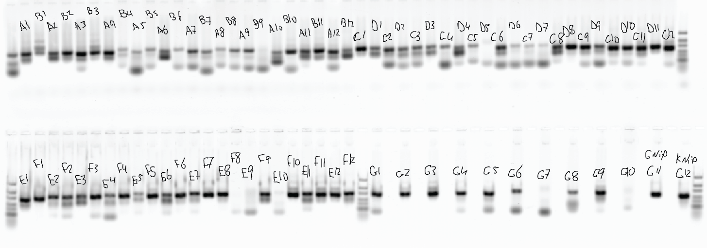
• Not all wells look good (see gel below), negative controls have bands.
• sequence, see what comes with the negative controls, see if we get any representation from the libraries without bands.
• Gel:
  

PCR to add NEB adaptors

• Samples: A1, C5, E6, F3, F5, G3, E2, F2, pool1, pool2 (2 uL of each)
• dilute 1:10 each adaptor sequence.
• to each: add 1.25 uL T7-adaptor, 1.25 uL common-adaptor, 12.5 uL 2x Phusion, 12.5 uL ddH2O
• 11x master = 13.75 T7-adaptor, 13.75 ul common, 137.5 uL Phusion, 137.5 uL ddH2O, 23 uL each.
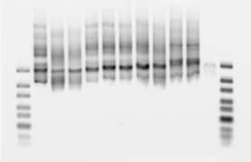
• 30 cycles NEB primers added (should have cut to like 10 cycles with this much template)
  

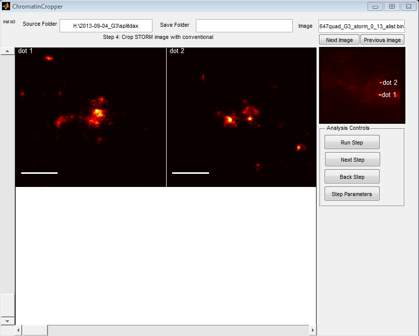
Coding chromatin region analysis GUI

Goals

• parse all conventional images to ID spots. Add filter to exclude out of focus spots and junk.
• extract spot image and molecule lists corresponding to conventional spots
• save
  1. spot conventional image,
  2. spot STORM image
  3. spot molecule list
  4. spot summary statistics (density, density regions)

Steps

1. Load conventional image
2. extract spot from conventional image
3. Load STORM data
4. Drift correct data, use conventional as filter to ID spots. Print a bunch of image views
5. save data for selected dots

Initial implementation

• single color
  

Project2

• helping Hao with matlab coding to cuts on regionprops
• working out 6 bit experiments

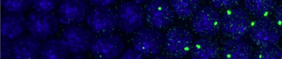
STORM imaging

• Imaging sample D09
• spots look good. 100% of cells have spots (size 18kb). Let’s see if we can get this size lower. Not bad for a non-transcribed region.
• also imaging Dm01-488 (direct label). Conventional looks good. STORM looks like nothing at all (not needed though).